Tobii eyetracking data from scratch • littlelisteners

In this example, I am going to produce a plot of proportion of looks to a target image for a block of eyetracking data, more or less, from scratch. The experiment was performed using Eprime with a Tobii eyetracker running at 60 FPS. The files for this experiment are bundled with this package and can be located with example_files().

library(tidyverse)
library(littlelisteners)
paths_to_block1 <- example_files(2)
basename(paths_to_block1)
#> [1] "Coartic_Block2_001P00XS1.gazedata" "Coartic_Block2_001P00XS1.txt"     
#> [3] "Coartic.yaml"

Where

the .gazedata file contains frame-by-frame eyetracking data.
the .txt filecontains Eprime’s trial-by-trial log of experiment data.
the .yaml file is a hand-created file with metadata about the experiment.

Reading in data

The experiment is a two-image looking-while-listening design. The yaml file includes the locations of the experiment’s areas of interest (AOIs) and the names of some pertinent fields to pull from the Eprime file.

data_yaml <- yaml::read_yaml(paths_to_block1[3])
str(data_yaml)
#> List of 5
#>  $ task     : chr "Coartic"
#>  $ notes    : chr "Coartic_WFFArea_2a (March 2013--ongoing).\nThe updated coarticulation pilot experiment incorporated \"filler\" "| __truncated__
#>  $ display  :List of 5
#>   ..$ type          : chr "Tobii60XL"
#>   ..$ frames_per_sec: num 60
#>   ..$ width_pix     : int 1920
#>   ..$ height_pix    : int 1200
#>   ..$ pixels_per_mm : num 3.71
#>  $ aois     :List of 3
#>   ..$ comment: chr "Describes the location of the onscreen areas of interest (AOIs) with respect to the screen origin. The AOIs are"| __truncated__
#>   ..$ ImageL :List of 8
#>   .. ..$ name    : chr "ImageL"
#>   .. ..$ x_length: int 600
#>   .. ..$ y_length: int 600
#>   .. ..$ x_limits: int [1:2] 100 700
#>   .. ..$ y_limits: int [1:2] 300 900
#>   .. ..$ x_origin: chr "left"
#>   .. ..$ y_origin: chr "bottom"
#>   .. ..$ units   : chr "pixels"
#>   ..$ ImageR :List of 8
#>   .. ..$ name    : chr "ImageR"
#>   .. ..$ x_length: int 600
#>   .. ..$ y_length: int 600
#>   .. ..$ x_limits: int [1:2] 1220 1820
#>   .. ..$ y_limits: int [1:2] 300 900
#>   .. ..$ x_origin: chr "left"
#>   .. ..$ y_origin: chr "bottom"
#>   .. ..$ units   : chr "pixels"
#>  $ locations:List of 2
#>   ..$ comment: chr "Names of the Eprime columns that say where each image is"
#>   ..$ target : chr "TargetImage"

data_yaml$notes |> 
  strwrap(70) |> 
  writeLines()
#> Coartic_WFFArea_2a (March 2013--ongoing). The updated coarticulation
#> pilot experiment incorporated "filler" trials and varied Pitch in the
#> carrier phrase. There is just one AudioStim file (2190 ms), with the
#> following parts: 1. Carrier word (find): 780 ms, 2. the: 560 ms, 3.
#> Target (ball): 850 ms. Target-onset occurs 1340 ms after
#> AudioStim.OnsetTime.

This yaml file is useful because it prevents me from having to some numbers.

The Eprime file format is a headache, but I made the rprime package to help clean wrangle them. It was my first R package so the function names are kind of clunky.

# install.packages("rprime")
data_trial_all <- rprime::read_eprime(paths_to_block1[2]) |> 
  rprime::FrameList() |> 
  rprime::filter_in("Eprime.Level", 3) |> 
  rprime::to_data_frame() |> 
  tibble::as_tibble()
data_trial_all
#> # A tibble: 24 × 34
#>    Eprime.Level Eprime.LevelName Eprime.Basename    Eprime.FrameNumber Procedure
#>           <dbl> <chr>            <chr>              <chr>              <chr>    
#>  1            3 TrialList_1      Coartic_Block2_00… 2                  TrialPro…
#>  2            3 TrialList_2      Coartic_Block2_00… 3                  TrialPro…
#>  3            3 TrialList_3      Coartic_Block2_00… 4                  TrialPro…
#>  4            3 TrialList_4      Coartic_Block2_00… 5                  TrialPro…
#>  5            3 TrialList_5      Coartic_Block2_00… 6                  TrialPro…
#>  6            3 TrialList_6      Coartic_Block2_00… 7                  TrialPro…
#>  7            3 TrialList_7      Coartic_Block2_00… 9                  TrialPro…
#>  8            3 TrialList_8      Coartic_Block2_00… 10                 TrialPro…
#>  9            3 TrialList_9      Coartic_Block2_00… 11                 TrialPro…
#> 10            3 TrialList_10     Coartic_Block2_00… 12                 TrialPro…
#> # ℹ 14 more rows
#> # ℹ 29 more variables: Running <chr>, ImageL <chr>, ImageR <chr>,
#> #   Carrier <chr>, Target <chr>, Pitch <chr>, AudioStim <chr>, Attention <chr>,
#> #   AudioDur <chr>, AttentionDur <chr>, WordGroup <chr>, StimType <chr>,
#> #   TargetWord <chr>, Cycle <chr>, Sample <chr>, Image2sec.OnsetTime <chr>,
#> #   Image2sec.StartTime <chr>, Fixation.OnsetDelay <chr>,
#> #   Fixation.OnsetTime <chr>, Fixation.StartTime <chr>, …

That has a lot of information. We can get to the core of the experiment’s trial data:

data_trial <- data_trial_all |> 
  rename_with(
    function(x) stringr::str_replace(x, ".OnsetTime", "Onset")
  ) |> 
  rename(CarrierOnset = TargetOnset) |> 
  mutate(
    across(c(ends_with("Onset"), AudioDur), as.numeric),
    TargetOnset = as.numeric(CarrierOnset) + 1340,
    TrialNo = Eprime.LevelName |> 
      stringr::str_extract("\\d+$") |> 
      as.numeric()
  ) |> 
  select(
    Basename = Eprime.Basename,
    TrialNo,
    Condition = StimType,
    WordGroup,
    TargetWord, 
    Target,
    AudioDur,
    Image2secOnset, 
    FixationOnset, 
    CarrierOnset, 
    TargetOnset, 
    Wait1SecFirstOnset, 
    AttentionOnset
  ) 
data_trial |> 
  glimpse()
#> Rows: 24
#> Columns: 13
#> $ Basename           <chr> "Coartic_Block2_001P00XS1", "Coartic_Block2_001P00X…
#> $ TrialNo            <dbl> 1, 2, 3, 4, 5, 6, 7, 8, 9, 10, 11, 12, 13, 14, 15, …
#> $ Condition          <chr> "neutral", "competing", "filler", "neutral", "facil…
#> $ WordGroup          <chr> "dog-book", "duck-ball", "cookie-shoe", "dog-book",…
#> $ TargetWord         <chr> "book", "duck", "cookie", "dog", "ball", "book", "c…
#> $ Target             <chr> "ImageL", "ImageR", "ImageL", "ImageR", "ImageR", "…
#> $ AudioDur           <dbl> 2190, 2190, 2190, 2190, 2190, 2190, 2190, 2190, 219…
#> $ Image2secOnset     <dbl> 32797, 41675, 60902, 70750, 80079, 91799, 105526, 1…
#> $ FixationOnset      <dbl> 34352, 43230, 62457, 72304, 81651, 93354, 107081, 1…
#> $ CarrierOnset       <dbl> 35087, 53412, 63560, 72940, 84426, 93856, 107565, 1…
#> $ TargetOnset        <dbl> 36427, 54752, 64900, 74280, 85766, 95196, 108905, 1…
#> $ Wait1SecFirstOnset <dbl> 37277, 55602, 65750, 75130, 86616, 96046, 109756, 1…
#> $ AttentionOnset     <dbl> 38281, 56605, 66754, 76133, 87619, 97049, 110759, 1…

Finally, we have the actual eyetracking data. read_gazedata() reads the .gazedata file into R as a tibble, applies some adjustments based on Tobii’s validity coding system, blanks out invalid gaze locations, flips the y measurements so the origin is the lower-left corner of the screen, and computes monocular means of eyetracking measurements.

data <- read_gazedata(paths_to_block1[1])
glimpse(data)
#> Rows: 15,265
#> Columns: 17
#> $ Basename      <chr> "Coartic_Block2_001P00XS1", "Coartic_Block2_001P00XS1", …
#> $ TrialNo       <int> 1, 1, 1, 1, 1, 1, 1, 1, 1, 1, 1, 1, 1, 1, 1, 1, 1, 1, 1,…
#> $ TobiiTime     <dbl> 1.360681e+12, 1.360681e+12, 1.360681e+12, 1.360681e+12, …
#> $ Time          <int> 32789, 32805, 32821, 32840, 32853, 32875, 32905, 32905, …
#> $ Origin        <chr> "LowerLeft", "LowerLeft", "LowerLeft", "LowerLeft", "Low…
#> $ XLeft         <dbl> 0.3590417, 0.3615159, 0.3729760, 0.3781238, 0.3811296, N…
#> $ XRight        <dbl> 0.3945794, 0.3814535, 0.3910438, 0.3896946, 0.3774196, N…
#> $ XMean         <dbl> 0.3768106, 0.3714847, 0.3820099, 0.3839092, 0.3792746, N…
#> $ YLeft         <dbl> 0.2779693, 0.2805615, 0.2833572, 0.2859311, 0.3208762, N…
#> $ YRight        <dbl> 0.2553138, 0.2349956, 0.2570407, 0.2132781, 0.2432799, N…
#> $ YMean         <dbl> 0.2666416, 0.2577785, 0.2701989, 0.2496046, 0.2820780, N…
#> $ ZLeft         <dbl> 542.9340, 542.9340, 543.7443, 543.7443, 544.3433, NA, NA…
#> $ ZRight        <dbl> 528.3995, 528.2514, 528.1776, 528.1776, 528.0162, NA, NA…
#> $ ZMean         <dbl> 535.6667, 535.5927, 535.9609, 535.9609, 536.1798, NA, NA…
#> $ DiameterLeft  <dbl> 3.846870, 3.638104, 3.692146, 3.343456, 3.469087, NA, NA…
#> $ DiameterRight <dbl> 3.627839, 3.651085, 3.590531, 3.453871, 3.542747, NA, NA…
#> $ DiameterMean  <dbl> 3.737354, 3.644595, 3.641338, 3.398664, 3.505917, NA, NA…

Note that the gaze locations are written in terms of screen proportions, not pixels where 0 is a bottom or left edge and 1 is a top or right edge.

Combining looking data and trial data

The Basename and TrialNo columns allow us to combine two dataframes.

data <- data |> 
  left_join(data_trial, by = c("Basename", "TrialNo"))

Now, we do a flurry of things. First, we define areas of interest and map looks to the AOIs.

aois <- list(
  create_aoi(
    aoi_name = data_yaml$aois$ImageL$name,
    x_pix = data_yaml$aois$ImageL$x_limits, 
    y_pix = data_yaml$aois$ImageL$y_limits,
    screen_width = data_yaml$display$width_pix,
    screen_height = data_yaml$display$height_pix
  ),
  create_aoi(
    aoi_name = data_yaml$aois$ImageR$name,
    x_pix = data_yaml$aois$ImageR$x_limits, 
    y_pix = data_yaml$aois$ImageR$y_limits,
    screen_width = data_yaml$display$width_pix,
    screen_height = data_yaml$display$height_pix
  )
)

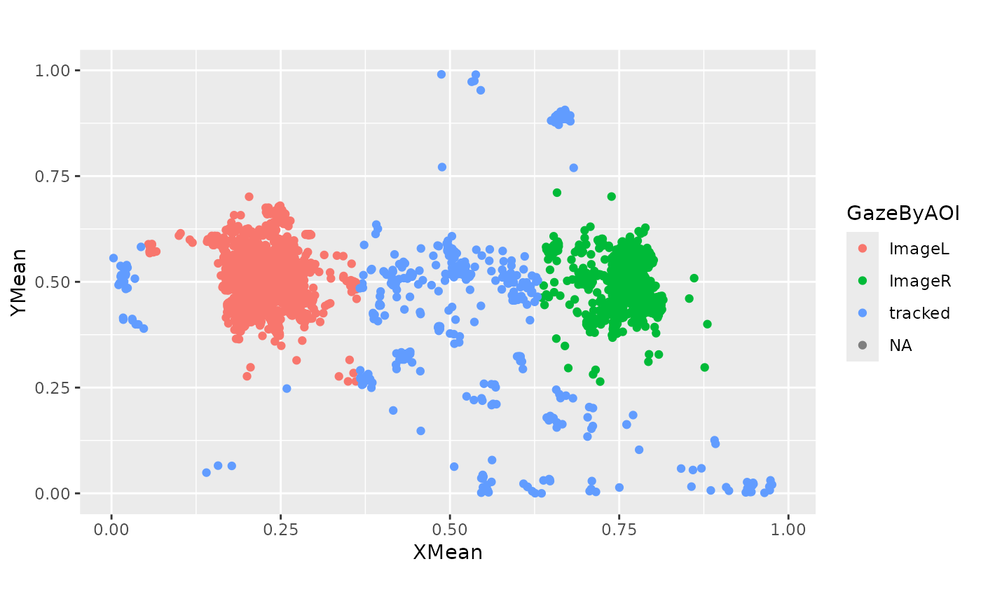
add_aois() maps from screen proportions to AOI locations. This function could use some work. It assumes that the looks are stored in XMean and YMean columns and creates a GazeByAOI column. It marks any onscreen look outside of an AOI as "tracked".

data <- data |> 
  add_aois(aois = aois, default_onscreen = "tracked")

ggplot(data) + 
  aes(x = XMean, y = YMean) + 
  geom_point(aes(color = GazeByAOI)) +
  coord_fixed(1200 / 1920)
#> Warning: Removed 11145 rows containing missing values or values outside the scale range
#> (`geom_point()`).

We can interpolate missing looks to remove blinks or other short gaps in the data. This will just fill in the response_col values and not the gaze locations.

data <- data |> 
  group_by(Basename, TrialNo) |> 
  interpolate_looks(
    window = 150, 
    fps = 60, 
    response_col = "GazeByAOI", 
    interp_col = "WasInterpolated", 
    fillable = c("ImageL", "ImageR"), 
    missing_looks = NA
  ) |> 
  ungroup()

Here is what we recovered:

data |> 
  count(GazeByAOI, WasInterpolated)
#> # A tibble: 6 × 3
#>   GazeByAOI WasInterpolated     n
#>   <chr>     <lgl>           <int>
#> 1 ImageL    FALSE            2739
#> 2 ImageL    TRUE              458
#> 3 ImageR    FALSE             927
#> 4 ImageR    TRUE              172
#> 5 tracked   FALSE             454
#> 6 NA        FALSE           10515

Now we map the left/right image locations GazeByAOI to the experimental roles of the images GazeByImageAOI in each trial. The least clever way to do this is a table join.

aoi_mapping <- tibble::tribble(
  ~GazeByAOI, ~Target, ~GazeByImageAOI,
  "ImageL",  "ImageL", "Target",
  "ImageL",  "ImageR", "Distractor",
  "ImageR",  "ImageR", "Target",
  "ImageR",  "ImageL", "Distractor",
  "tracked", "ImageL", "tracked",
  "tracked", "ImageR", "tracked",
  NA,  "ImageL", NA,
  NA, "ImageR", NA
)

data <- data |> 
  left_join(aoi_mapping, by = c("Target", "GazeByAOI"))

The final step for preprocessing is to align the trials so that time = 0 is the target onset. This function should just work on grouped dataframe sigh instead of including them haphazardly.

data <- data |> 
  adjust_times(
    time_var = Time, event_var = TargetOnset, 
    # grouping variables
    Basename, TrialNo
  )

Aggregating data

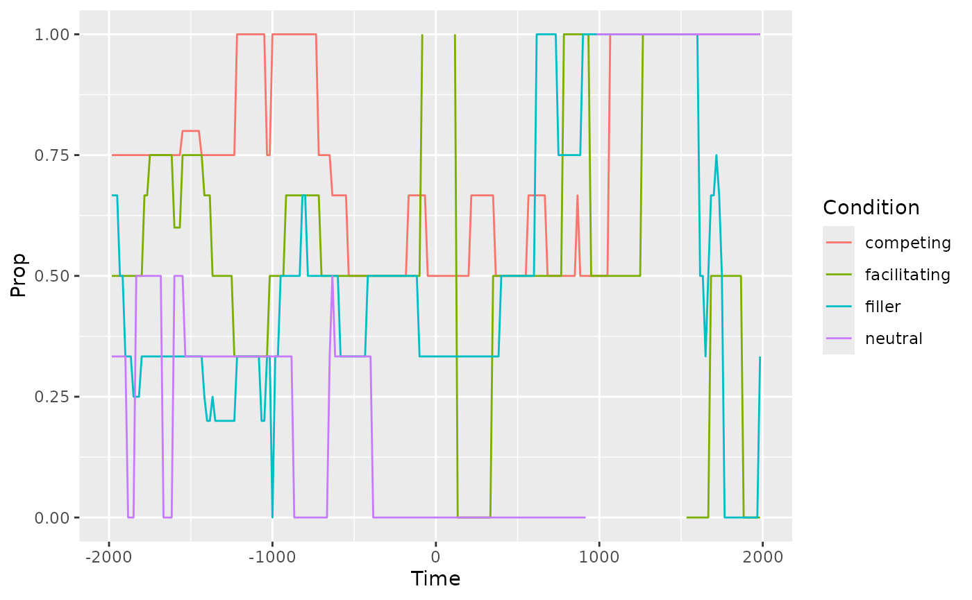
At each frame, we can count the proportion of looks to the target. First, we need create a response definition which tells little listeners how to treat the labels in terms of targets and competitors.

def <- create_response_def(
  primary = "Target", 
  others = "Distractor", 
  elsewhere = "tracked"
)

data_agg <- data |> 
  filter(-2000 < Time, Time < 2000) |> 
  aggregate_looks(def, Condition + Time ~ GazeByImageAOI)

ggplot(data_agg) + 
  aes(x = Time, y = Prop) +
  geom_line(aes(color = Condition))

From here, we might combine multiple blocks of trials for this participant together and downsample the data into 50 ms to get a less jumpy line.